Counterfactual Regret
Motivation
This project was an attempt to work through An Introduction to Counterfactual Regret Minimization of Todd W. Neller and Marc Lanctot to have a better understanding on how strategies are found.
To be honest, it was also a way to learn how to find optimal strategies on boardgames.
Content
This project covers two examples of normal-form games: Rock-Paper-Scissor and Colonel Blotto. While RPS was a simple example to learn the basics, Colonel Blotto is a more complicated (while still being played in a single simultaneous turn).
Objective
The aim of this implementation is to find an optimal (mixed) strategy using CFR and monte-carlo sampling which consists of four parts:
- computing utility of all pure strategies
- draw a random action
- accumulate regret
- compute average strategies
Then steps 2 to 4 are repeted several times to achieve convergence.
If you need more information about these steps, you can find valuable information in the linked PDF.
Example: RPS
It is expected there is no optimal strategy in RPS aside a random one. The solver finds the following optimal strategy:
Executing Monte-Carlo CFR for 100000 steps with seed 1
Nash strategies :
Action    player 1        player 2
ROCK      0.3347622       0.3366166
PAPER     0.3332283       0.3311550
SCISSOR   0.3320096       0.3322284
which is consistant which the theory. Thanks to this little project, I will be a better RPS player.
Example: Colonel Blotto
Rules
Colonel Blotto is a simple game. There are B battlefields and each player has S soldiers that they will simultaneously place. Then for each battlefield, the player with the most soldiers will win it, and the winner will be the one that wins the most battlefields.
Some obviously bad strategies is to place all soldiers in one battlefield. Of course you will win it, but you will loose all other ones (which is bad if there are more than 2 battlefields).
Counting
While the bulk of the algorithm is still the same, the main difficulty here is to count all pure strategies. One can show there are \({B+S-1\choose B-1}\) pure strategies (it’s a star and bar problem). At first, I use algorithm T from The Art Of Computer Programming, Volume 4A, Third Edition, which computes all lexicographic combinations. The project includes two implementations of such algorithm, one using goto statement that mirrors the pseudo-code, and another one that doesn’t use any goto statement.
However, I ended up using a combinatorial number system since encoding a combination on a uint16 means I can go up to 18 battlefields+soldiers. Whereas exploring the same combination using algorithm T means using an array of uint16 (of size B-1), which is memory intensive.
Results
For a Colonel Blotto with 3 battlefields and 5 soldiers, the solver finds the following optimal strategy:
Executing Monte-Carlo CFR for 100000 steps with seed 1
Nash strategies :
Action         player 1        player 2
0, 0, 5,       0.0000005       0.0000005
0, 1, 4,       0.0000005       0.0000562
1, 0, 4,       0.0000171       0.0000296
0, 2, 3,       0.1134408       0.1255362
1, 1, 3,       0.1127920       0.0959764
2, 0, 3,       0.1123847       0.1199302
0, 3, 2,       0.0992561       0.1042694
1, 2, 2,       0.0000380       0.0000024
2, 1, 2,       0.0000119       0.0000258
3, 0, 2,       0.1110097       0.1162245
0, 4, 1,       0.0000026       0.0000182
1, 3, 1,       0.1264002       0.1136648
2, 2, 1,       0.0000371       0.0000433
3, 1, 1,       0.1181154       0.1013618
4, 0, 1,       0.0000093       0.0000461
0, 5, 0,       0.0000005       0.0000005
1, 4, 0,       0.0000274       0.0000420
2, 3, 0,       0.1009886       0.1057043
3, 2, 0,       0.1054664       0.1170096
4, 1, 0,       0.0000007       0.0000577
5, 0, 0,       0.0000005       0.0000005
As expected, the (5, 0, 0)-like strategies (placing 5 soldiers in one battlefield and none on the others) are bad, as well as the (4, 1, 0)-like and the (2, 2, 1)-like strategies. At the opposite, the (3, 2, 0)-like and (3, 1, 1)-like are the best ones.
Seed-dependance ?
Since there are multiple possible Nash equilibrium in the set-up (degenerate game), some actions could be discarded by the solver and it may not return the fully mixed strategy. Here is an example of an optimal strategies with 2 soldiers and 3 battlefields:
Executing Monte-Carlo CFR for 100000 steps with seed 1
Nash strategies :
Action         player 1        player 2
0, 0, 2,       0.0000033       0.0000100
0, 1, 1,       0.1667241       0.9999500
1, 0, 1,       0.4998119       0.0000100
0, 2, 0,       0.0000097       0.0000100
1, 1, 0,       0.3334399       0.0000100
2, 0, 0,       0.0000111       0.000010
Here player 2 will always pick the strategy (0, 1, 1) and will discard (1, 0, 1) and (1, 1, 0) while they all give the same utility against player 1. Using the same step up but with different seeds will lead to different outcome:
Executing Monte-Carlo CFR for 100000 steps with seed 10
Nash strategies :
Action         player 1        player 2
0, 0, 2,       0.0000033       0.0000183
0, 1, 1,       0.0000215       0.0000183
1, 0, 1,       0.0000215       0.4999633
0, 2, 0,       0.0000115       0.0000183
1, 1, 0,       0.9999369       0.4999633
2, 0, 0,       0.0000053       0.0000183
It’s a non-issue. In fact the two differents optimal strategies from seed 1 and 10 are optimal. This result appears because of early attraction and sampling.
Convergence vizualisation
The project comes with a python script that can be used for generating animated gif from the exported average strategies.
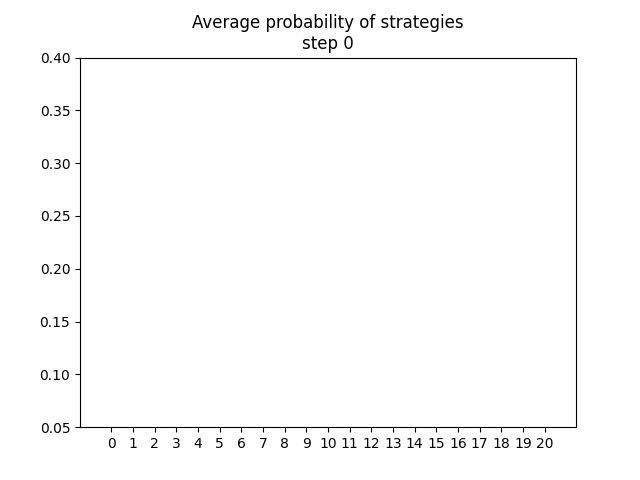
Here, strategy 0 is (0, 0, 5,), strategy 1 is (0, 1, 4,) and so on. The full list of all strategies are found earlier.
Next steps
Currently the goal of this exploration is achieved but I may add more examples of simultaneous games. It’s unlikely, I want to focus on learning how to solve sequential games instead.
Unless I found a bug or I want to improve the gif export with titles and better naming, this project is “on-hold”. It was fun.